Deep Learning: From Basics to Advanced Concepts

Muhammad Abdullah - AI/ML Engineer

Table of Contents

1. Introduction to Deep Learning
2. Neural Networks
   • Perceptron
   • Artificial Neural Networks (ANNs)
   • How ANNs Work
   • Activation Functions
   • Optimization
3. Forward Propagation and Backward Propagation
   • Forward Propagation
   • Backward Propagation
   • Gradient Descent
   • Vanishing Gradient Problem
4. Loss Functions
   • Types of Loss Functions
   • When to Use Which Loss Function
5. Convolutional Neural Networks (CNNs)
   • Convolution Operation
   • Pooling
   • Fully Connected Layer
6. R-CNN (Region-based Convolutional Neural Networks)
   • Architecture
   • Workflow
   • Limitations
7. Fast R-CNN
   • Architecture
   • Workflow
   • Improvements over R-CNN
8. Faster R-CNN
   • Region Proposal Network (RPN)
   • Architecture
   • Workflow
   • Improvements over Fast R-CNN
9. Mask R-CNN
   • Architecture
   • Workflow
   • Loss Function
   • RoIAlign
   • Applications and Experiments
   • Limitations and Future Work
10. Recurrent Neural Networks (RNNs)
    • Architecture
    • Types of RNNs
    • Applications
11. Long Short-Term Memory (LSTM) Networks
    • Architecture
    • Workflow
    • Applications
12. Generative Adversarial Networks (GANs)
    • Architecture
    • Workflow
    • Applications
13. Conclusion
14. Appendix: Mapping Table

Introduction to Deep Learning

Deep learning is a subset of machine learning that uses artificial neural networks with many layers to model and understand complex patterns in data. It has revolutionized various fields, including computer vision, natural language processing, and speech recognition.

Key Concepts

• Neural Networks: Inspired by the human brain, neural networks consist of interconnected layers of nodes (neurons) that process information.
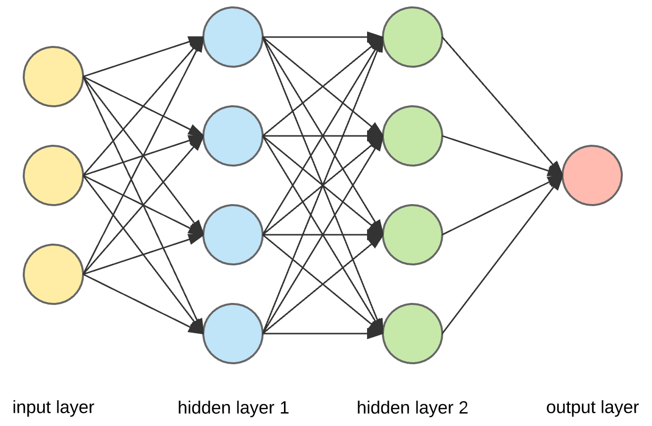
• Layers: Neural networks are composed of multiple layers, including input, hidden, and output layers.
• Training: The process of adjusting the weights of the neural network to minimize the error between predicted and actual outputs.

Neural Networks

Figure: A typical neural network architecture showing input layer (left), hidden layers (middle), and output layer (right). Source: Wikimedia Commons

Perceptron

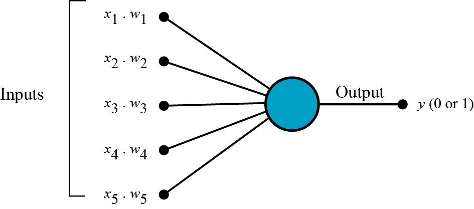
The perceptron is the simplest form of a neural network, introduced by Frank Rosenblatt in 1957. It consists of a single layer of weights that connect inputs to an output.

• Input: $ x_1, x_2, \ldots, x_n $
• Weights: $ w_1, w_2, \ldots, w_n $
• Bias: $ b $
• Output: $ y $

The output of a perceptron is given by:

$$ y = f\left(\sum_{i=1}^{n} w_i x_i + b\right) $$

where $ f $ is an activation function. Figure: Perceptron architecture showing inputs (x1, x2), weights (w1, w2), bias (b), and activation function (f). Source: Medium

Figure: Perceptron decision boundary separating two classes in 2D space. Source: Medium

Artificial Neural Networks (ANNs)

Artificial Neural Networks (ANNs) are more complex models that consist of multiple layers of interconnected neurons. They can model complex relationships in data.

How ANNs Work

ANNs work by passing inputs through layers of neurons, where each neuron performs a weighted sum of its inputs, adds a bias, and applies an activation function.

• Input Layer: Receives the input data.
• Hidden Layers: Process the input data through multiple layers of neurons.
• Output Layer: Produces the final output.

The output of a neuron in a hidden layer is given by:

$$ z_j = f\left(\sum_{i=1}^{n} w_{ji} x_i + b_j\right) $$

where $ z_j $ is the output of the $ j $-th neuron, $ w_{ji} $ are the weights, $ x_i $ are the inputs, $ b_j $ is the bias, and $ f $ is the activation function.

Activation Functions

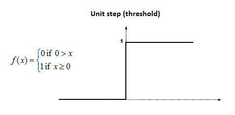
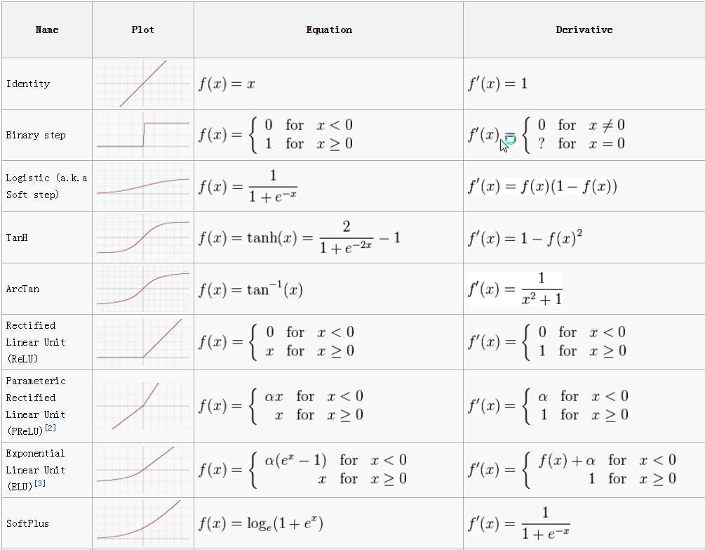
Activation functions introduce non-linearity into the model, allowing it to learn complex patterns. Common activation functions include:

• Sigmoid: $ \sigma(x) = \frac{1}{1 + e^{-x}} $
  • Use Case: Often used in the output layer for binary classification problems.
• Tanh: $ \tanh(x) = \frac{e^x - e^{-x}}{e^x + e^{-x}} $
  • Use Case: Used in hidden layers to introduce non-linearity.
• ReLU (Rectified Linear Unit): $ \text{ReLU}(x) = \max(0, x) $
  • Use Case: Widely used in hidden layers for its simplicity and effectiveness in deep networks.
• Leaky ReLU: $ \text{Leaky ReLU}(x) = \max(0.01x, x) $
  • Use Case: Used to mitigate the dying ReLU problem, where neurons can get stuck in the negative region.
• Softmax: $ \text{Softmax}(x_i) = \frac{e^{x_i}}{\sum_{j} e^{x_j}} $
  • Use Case: Used in the output layer for multi-class classification problems.

Optimization

Optimization involves adjusting the weights of the neural network to minimize the loss function. Common optimization algorithms include:

• Gradient Descent: Updates the weights in the direction of the negative gradient of the loss function.
  • Use Case: Basic optimization algorithm, but can be slow for large datasets.
• Stochastic Gradient Descent (SGD): Updates the weights using a single training example at a time.
  • Use Case: Faster than gradient descent, but can be noisy.
• Mini-batch Gradient Descent: Updates the weights using a small batch of training examples.
  • Use Case: Balances the speed of SGD and the stability of gradient descent.
• Adam: An adaptive learning rate optimization algorithm that combines the benefits of two other extensions of stochastic gradient descent.
  • Use Case: Widely used for its efficiency and effectiveness in training deep networks.

The weight update rule for gradient descent is given by:

$$ w_{ij} := w_{ij} - \eta \frac{\partial L}{\partial w_{ij}} $$

where $ \eta $ is the learning rate, $ L $ is the loss function, and $ \frac{\partial L}{\partial w_{ij}} $ is the gradient of the loss with respect to the weight $ w_{ij} $.

Visual Illustrations

1. Neural Network Architecture Basic architecture of an artificial neural network showing input layer, hidden layers, and output layer

2. Activation Functions Visualization of common activation functions: Sigmoid, Tanh, ReLU, and Leaky ReLU

3. Optimization Process Gradient descent optimization process showing how weights are updated to minimize loss

4. Forward Propagation Forward propagation process showing how input signals propagate through the network

5. Backward Propagation Backward propagation process showing how errors propagate backwards through the network

Forward Propagation and Backward Propagation

Forward Propagation

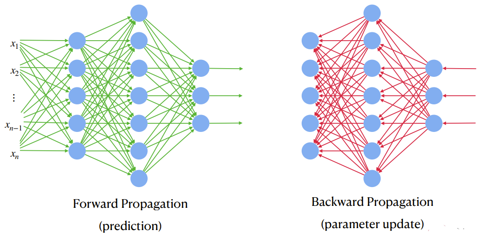
Forward propagation is the process of passing input data through the neural network to generate an output. It involves the following steps:

1. Input Layer: Receive the input data.
2. Hidden Layers: Compute the weighted sum of inputs, add the bias, and apply the activation function for each neuron.
3. Output Layer: Generate the final output.

The output of a neuron in a hidden layer is given by:

$$ z_j = f\left(\sum_{i=1}^{n} w_{ji} x_i + b_j\right) $$

Backward Propagation

Backward propagation is the process of adjusting the weights of the neural network to minimize the loss function. It involves the following steps:

1. Compute the Loss: Calculate the loss between the predicted and actual outputs.
2. Compute the Gradient: Calculate the gradient of the loss with respect to each weight using the chain rule.
3. Update the Weights: Adjust the weights in the direction of the negative gradient.

The weight update rule for gradient descent is given by:

$$ w_{ij} := w_{ij} - \eta \frac{\partial L}{\partial w_{ij}} $$

Gradient Descent

Gradient descent is an optimization algorithm that adjusts the weights of the neural network to minimize the loss function. It involves the following steps:

1. Initialize the Weights: Start with random initial weights.
2. Compute the Gradient: Calculate the gradient of the loss with respect to each weight.
3. Update the Weights: Adjust the weights in the direction of the negative gradient.
4. Repeat: Repeat the process until the loss converges.

Vanishing Gradient Problem

The vanishing gradient problem occurs when the gradients become very small in the early layers of the network, making it difficult to update the weights. This can slow down the training process and make it difficult to learn long-term dependencies.

• Cause: Activation functions like sigmoid and tanh can squash the gradients to very small values.
• Solution: Use activation functions like ReLU, which do not suffer from the vanishing gradient problem.

Loss Functions

Loss functions measure the difference between the predicted and actual outputs. They guide the optimization process by providing a signal for adjusting the weights.

Types of Loss Functions

1. Mean Squared Error (MSE) Loss:

   • Formula: $ L = \frac{1}{n} \sum_{i=1}^{n} (y_i - \hat{y}_i)^2 $
   • Use Case: Regression problems.

2. Cross-Entropy Loss:

   • Formula: $ L = -\frac{1}{n} \sum_{i=1}^{n} [y_i \log(\hat{y}_i) + (1 - y_i) \log(1 - \hat{y}_i)] $
   • Use Case: Binary classification problems.

3. Categorical Cross-Entropy Loss:

   • Formula: $ L = -\frac{1}{n} \sum_{i=1}^{n} \sum_{j=1}^{m} y_{ij} \log(\hat{y}_{ij}) $
   • Use Case: Multi-class classification problems.

4. Hinge Loss:

   • Formula: $ L = \max(0, 1 - y_i \hat{y}_i) $
   • Use Case: Support Vector Machines (SVMs).

5. Huber Loss:

   • Formula: $ L = \begin{cases} \frac{1}{2} (y_i - \hat{y}_i)^2 & \text{if } |y_i - \hat{y}_i| \leq \delta \ \delta (|y_i - \hat{y}_i| - \frac{1}{2} \delta) & \text{otherwise} \end{cases} $
   • Use Case: Robust regression problems.

When to Use Which Loss Function

Loss Function	Use Case
Mean Squared Error (MSE) Loss	Regression problems
Cross-Entropy Loss	Binary classification problems
Categorical Cross-Entropy Loss	Multi-class classification problems
Hinge Loss	Support Vector Machines (SVMs)
Huber Loss	Robust regression problems

Convolutional Neural Networks (CNNs)

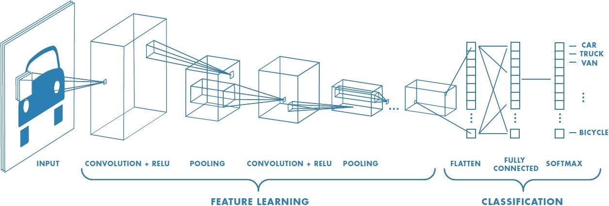
Convolutional Neural Networks (CNNs) are a type of deep learning model specifically designed for processing structured grid data like images. They use convolution operations to automatically and adaptively learn spatial hierarchies of features.

Convolution Operation

The convolution operation involves a filter (or kernel) that slides over the input image to produce a feature map.

• Filter/Kernel: A small matrix of weights that is used to detect specific features in the input image.
• Stride: The number of pixels by which the filter moves over the image.

The output of a convolution operation is given by:

$$ (I * K)(i, j) = \sum_{m} \sum_{n} I(i + m, j + n) K(m, n) $$

where $ I $ is the input image, $ K $ is the filter, and $ * $ denotes the convolution operation.

Figure: Animation showing how a convolution filter slides over an input image to produce a feature map. Source: Medium

Pooling

Pooling is a down-sampling operation that reduces the spatial dimensions of the feature map, retaining the most important information and reducing the computational load.

• Max Pooling: Takes the maximum value from a patch of the feature map.
• Average Pooling: Takes the average value from a patch of the feature map.

Figure: Animation demonstrating max pooling operation with a 2x2 filter and stride of 2. The maximum value in each 2x2 region is selected for the output feature map. Source: Medium

Fully Connected Layer

After several convolutional and pooling layers, the high-level reasoning in the neural network is done via fully connected layers. Neurons in a fully connected layer have full connections to all activations in the previous layer.

The complete CNN architecture combines these components:

1. Convolutional Layers: Extract features using filters
2. Pooling Layers: Reduce spatial dimensions
3. Fully Connected Layers: Perform high-level reasoning

Figure: Complete CNN architecture showing the sequence of convolutional layers, pooling layers, and fully connected layers transforming an input image into class predictions. Source: Medium

R-CNN (Region-based Convolutional Neural Networks)

R-CNN is one of the pioneering works in object detection using deep learning. It was introduced by Ross Girshick et al. in 2014.

Architecture

R-CNN consists of three main components:

1. Region Proposal: Generates region proposals using selective search.
2. Feature Extraction: Extracts features from each region proposal using a pre-trained CNN.
3. Classification and Bounding Box Regression: Classifies each region proposal and refines the bounding box coordinates using SVMs and linear regression.

Workflow

1. Region Proposal:

   • Use selective search to generate around 2000 region proposals per image.

2. Feature Extraction:

   • Warp each region proposal to a fixed size (e.g., 224x224 pixels).
   • Pass each warped region through a pre-trained CNN (e.g., AlexNet) to extract features.

3. Classification and Bounding Box Regression:

   • Use SVMs to classify each region proposal.
   • Use linear regression to refine the bounding box coordinates.

Limitations

• Speed: R-CNN is slow because it processes each region proposal independently, leading to redundant computations.
• Training: The training process is multi-stage and complex, involving separate training for the CNN, SVMs, and bounding box regressors.
• Storage: Requires a large amount of storage to save the features for each region proposal.

Fast R-CNN

Fast R-CNN is an improvement over R-CNN, introduced by Ross Girshick in 2015. It addresses the speed and storage issues of R-CNN.

Architecture

Fast R-CNN consists of two main components:

1. Region Proposal: Generates region proposals using selective search or EdgeBoxes.
2. Region of Interest (RoI) Pooling: Projects the region proposals onto the feature map and pools the features.
3. Classification and Bounding Box Regression: Classifies each region proposal and refines the bounding box coordinates using a single network.

Workflow

1. Region Proposal:

   • Use selective search or EdgeBoxes to generate region proposals.

2. Feature Extraction:

   • Pass the entire image through a pre-trained CNN to extract a feature map.

3. RoI Pooling:

   • Project the region proposals onto the feature map.
   • Pool the features from each region proposal to a fixed size (e.g., 7x7).

4. Classification and Bounding Box Regression:

   • Pass the pooled features through fully connected layers to classify each region proposal and refine the bounding box coordinates.

Improvements over R-CNN

• Speed: Fast R-CNN is faster because it shares the computation of the feature map for all region proposals.
• Training: The training process is end-to-end, simplifying the training pipeline.
• Storage: Requires less storage because it does not need to save the features for each region proposal.

Faster R-CNN

Faster R-CNN is an improvement over Fast R-CNN, introduced by Shaoqing Ren et al. in 2015. It addresses the bottleneck of region proposal generation.

Region Proposal Network (RPN)

RPN is a fully convolutional network that predicts region proposals directly from the feature map. It consists of two main components:

1. Anchor Boxes: Pre-defined boxes of different sizes and aspect ratios.
2. Classification and Bounding Box Regression: Classifies each anchor box as foreground or background and refines the bounding box coordinates.

Architecture

Faster R-CNN consists of two main components:

1. Region Proposal Network (RPN): Generates region proposals from the feature map.
2. Fast R-CNN: Classifies each region proposal and refines the bounding box coordinates.

Workflow

1. Feature Extraction:

   • Pass the entire image through a pre-trained CNN to extract a feature map.

2. Region Proposal Network (RPN):

   • Slide a small network over the feature map to predict region proposals.
   • For each position in the feature map, predict the probability of each anchor box being foreground or background and refine the bounding box coordinates.

3. RoI Pooling:

   • Project the region proposals onto the feature map.
   • Pool the features from each region proposal to a fixed size (e.g., 7x7).

4. Classification and Bounding Box Regression:

   • Pass the pooled features through fully connected layers to classify each region proposal and refine the bounding box coordinates.

Improvements over Fast R-CNN

• Speed: Faster R-CNN is faster because it generates region proposals directly from the feature map, eliminating the need for external region proposal methods.
• Accuracy: The region proposals generated by RPN are more accurate because they are learned from the data.

Mask R-CNN

Mask R-CNN is an extension of Faster R-CNN for instance segmentation, introduced by Kaiming He et al. in 2017. It adds a branch for predicting segmentation masks on top of the existing branch for bounding box recognition.

Architecture

Mask R-CNN consists of three main components:

1. Region Proposal Network (RPN): Generates region proposals from the feature map.
2. RoIAlign: Aligns the region proposals to the feature map.
3. Mask Branch: Predicts segmentation masks for each region proposal.

Workflow

1. Feature Extraction:

   • Pass the entire image through a pre-trained CNN to extract a feature map.

2. Region Proposal Network (RPN):

   • Slide a small network over the feature map to predict region proposals.
   • For each position in the feature map, predict the probability of each anchor box being foreground or background and refine the bounding box coordinates.

3. RoIAlign:

   • Project the region proposals onto the feature map.
   • Align the region proposals to the feature map using bilinear interpolation to preserve spatial correspondence.

4. Mask Branch:

   • Pass the aligned features through a small fully convolutional network to predict segmentation masks for each region proposal.

5. Classification and Bounding Box Regression:

   • Pass the aligned features through fully connected layers to classify each region proposal and refine the bounding box coordinates.

Loss Function

The loss function for Mask R-CNN is a multi-task loss that combines the losses for classification, bounding box regression, and mask prediction:

$$ L = L_{cls} + L_{box} + L_{mask} $$

• $ L_{cls} $: Classification loss (cross-entropy loss).
• $ L_{box} $: Bounding box regression loss (smooth L1 loss).
• $ L_{mask} $: Mask prediction loss (binary cross-entropy loss).

RoIAlign

RoIAlign is a method for aligning the region proposals to the feature map. It addresses the quantization issue of RoIPool by using bilinear interpolation to compute the exact values of the input features. This preserves the spatial correspondence between the input and output features, leading to more accurate segmentation masks.

Applications and Experiments

Mask R-CNN has been applied to various tasks, including:

• Instance Segmentation: Delineating each object at a pixel level.
• Object Detection: Detecting and locating objects within an image.
• Robot Manipulation: Estimating object position for grasp planning.

Experiments on the COCO dataset have shown that Mask R-CNN outperforms previous state-of-the-art instance segmentation models by a large margin.

Limitations and Future Work

• Temporal Information: Mask R-CNN only works on images, so it cannot explore temporal information of objects in a dynamic setting.
• Motion Blur: Mask R-CNN usually suffers from motion blur at low resolution and encounters failures.
• Supervised Training: Mask R-CNN requires labeled data for training, which can be difficult to obtain.

Future work includes:

• Hand Segmentation: Combining Mask R-CNN with tracking for hand segmentation under different viewpoints.
• Embodied Amodal Recognition: Applying Mask R-CNN for agents to learn to move strategically to improve their visual recognition abilities.

Figure: Mask R-CNN workflow showing the stages from input image through region proposals, feature extraction, and final instance segmentation masks. The network simultaneously detects objects (bounding boxes), classifies them, and generates pixel-level segmentation masks. Source: Medium

Recurrent Neural Networks (RNNs)

Recurrent Neural Networks (RNNs) are a type of neural network designed for processing sequential data, such as time series or natural language. They have loops within their architecture that allow information to persist.

Architecture

RNNs consist of the following components:

1. Input Layer: Receives the input data.
2. Hidden Layer: Processes the input data and maintains a hidden state that captures information from previous time steps.
3. Output Layer: Produces the final output.

The hidden state at time step $ t $ is given by:

$$ h_t = f(W_h h_{t-1} + W_x x_t + b) $$

where $ h_t $ is the hidden state at time step $ t $, $ W_h $ and $ W_x $ are the weight matrices, $ x_t $ is the input at time step $ t $, $ b $ is the bias, and $ f $ is the activation function.

Types of RNNs

1. Simple RNN: The basic form of RNN with a single hidden layer.
2. LSTM (Long Short-Term Memory): A type of RNN designed to mitigate the vanishing gradient problem and capture long-term dependencies.
3. GRU (Gated Recurrent Unit): A simplified version of LSTM with fewer parameters.

Applications

• Natural Language Processing: Language modeling, machine translation, text generation.
• Time Series Analysis: Stock price prediction, weather forecasting.
• Speech Recognition: Converting spoken language into text.

Long Short-Term Memory (LSTM) Networks

Long Short-Term Memory (LSTM) networks are a type of RNN designed to capture long-term dependencies in sequential data. They introduce a memory cell and gates to control the flow of information.

Architecture

LSTM networks consist of the following components:

1. Input Gate: Controls the flow of input activations into the memory cell.
2. Forget Gate: Controls the flow of information from the previous time step into the memory cell.
3. Output Gate: Controls the flow of information from the memory cell to the output.
4. Memory Cell: Stores information over time.

The hidden state at time step $ t $ is given by:

$$ h_t = o_t \odot \tanh(C_t) $$

where $ h_t $ is the hidden state at time step $ t $, $ o_t $ is the output gate, $ C_t $ is the memory cell, and $ \odot $ denotes element-wise multiplication.

Workflow

1. Input Gate:

   • Compute the input gate activation: $ i_t = \sigma(W_i [h_{t-1}, x_t] + b_i) $
   • Compute the candidate memory cell: $ \tilde{C}t = \tanh(W_C [h{t-1}, x_t] + b_C) $

2. Forget Gate:

   • Compute the forget gate activation: $ f_t = \sigma(W_f [h_{t-1}, x_t] + b_f) $

3. Memory Cell:

   • Update the memory cell: $ C_t = f_t \odot C_{t-1} + i_t \odot \tilde{C}_t $

4. Output Gate:

   • Compute the output gate activation: $ o_t = \sigma(W_o [h_{t-1}, x_t] + b_o) $
   • Compute the hidden state: $ h_t = o_t \odot \tanh(C_t) $

Applications

• Natural Language Processing: Language modeling, machine translation, text generation.
• Time Series Analysis: Stock price prediction, weather forecasting.
• Speech Recognition: Converting spoken language into text.

Generative Adversarial Networks (GANs)

Generative Adversarial Networks (GANs) are a type of deep learning model designed for generating new data instances that resemble the training data. They consist of two networks: a generator and a discriminator.

Architecture

GANs consist of the following components:

1. Generator: Generates new data instances.
2. Discriminator: Distinguishes between real and generated data instances.

The generator and discriminator are trained simultaneously in a minimax game, where the generator tries to fool the discriminator, and the discriminator tries to correctly classify the data.

Workflow

1. Generator:

   • Generate new data instances: $ G(z) $
   • Update the generator weights to maximize the discriminator's error.

2. Discriminator:

   • Classify the data instances: $ D(x) $
   • Update the discriminator weights to minimize the classification error.

The loss function for GANs is given by:

$$ \min_G \max_D V(D, G) = \mathbb{E}{x \sim p{data}(x)}[\log D(x)] + \mathbb{E}_{z \sim p_z(z)}[\log(1 - D(G(z)))] $$

where $ G $ is the generator, $ D $ is the discriminator, $ x $ is the real data, $ z $ is the noise vector, $ p_{data}(x) $ is the data distribution, and $ p_z(z) $ is the noise distribution.

Applications

• Image Generation: Generating realistic images.
• Image Super-Resolution: Enhancing the resolution of images.
• Style Transfer: Transferring the style of one image to another.

Conclusion

Deep learning, with its foundations in neural networks, has revolutionized various fields by enabling the modeling of complex patterns in data. Neural networks, from simple perceptrons to complex architectures like CNNs, RNNs, LSTMs, and GANs, have paved the way for advanced models like R-CNN, Fast R-CNN, and Mask R-CNN. These models have significantly improved object detection, instance segmentation, sequential data processing, and data generation, making them invaluable tools in computer vision, natural language processing, and beyond.

This comprehensive understanding of deep learning, from the basics to advanced concepts, should give you a solid foundation in the field. If you have any specific questions or need further clarification on any topic, feel free to ask!

Appendix: Mapping Table

Activation Functions

Activation Function	Formula	Use Case
Sigmoid	$\sigma(x) = \frac{1}{1 + e^{-x}}$	Output layer for binary classification
Tanh	$\tanh(x) = \frac{e^x - e^{-x}}{e^x + e^{-x}}$	Hidden layers
ReLU	$\text{ReLU}(x) = \max(0, x)$	Hidden layers
Leaky ReLU	$\text{Leaky ReLU}(x) = \max(0.01x, x)$	Hidden layers to mitigate dying ReLU
Softmax	$\text{Softmax}(x_i) = \frac{e^{x_i}}{\sum_{j} e^{x_j}}$	Output layer for multi-class classification

Loss Functions

Loss Function	Formula	Use Case
Mean Squared Error (MSE) Loss	$L = \frac{1}{n} \sum_{i=1}^{n} (y_i - \hat{y}_i)^2$	Regression problems
Cross-Entropy Loss	$L = -\frac{1}{n} \sum_{i=1}^{n} [y_i \log(\hat{y}_i) + (1 - y_i) \log(1 - \hat{y}_i)]$	Binary classification problems
Categorical Cross-Entropy Loss	$L = -\frac{1}{n} \sum_{i=1}^{n} \sum_{j=1}^{m} y_{ij} \log(\hat{y}_{ij})$	Multi-class classification problems
Hinge Loss	$L = \max(0, 1 - y_i \cdot \hat{y}_i)$	Support Vector Machines (SVMs)

Optimization Algorithms

Optimization Algorithm	Description	Use Case
Gradient Descent	Updates the weights in the direction of the negative gradient of the loss function	Basic optimization, slow for large datasets
Stochastic Gradient Descent (SGD)	Updates the weights using a single training example at a time	Faster than gradient descent, but can be noisy
Mini-batch Gradient Descent	Updates the weights using a small batch of training examples	Balances speed and stability
Adam	Adaptive learning rate optimization algorithm	Efficient and effective for training deep networks

References

1. Goodfellow, I., Bengio, Y., & Courville, A. (2016). Deep Learning. MIT Press.
2. LeCun, Y., Bengio, Y., & Hinton, G. (2015). Deep learning. Nature, 521(7553), 436-444.
3. He, K., Gkioxari, G., Dollár, P., & Girshick, R. (2017). Mask R-CNN. IEEE International Conference on Computer Vision (ICCV).
4. Hochreiter, S., & Schmidhuber, J. (1997). Long Short-Term Memory. Neural Computation, 9(8), 1735-1780.
5. Krizhevsky, A., Sutskever, I., & Hinton, G. E. (2012). ImageNet Classification with Deep Convolutional Neural Networks. Advances in Neural Information Processing Systems.

Figure: Evolution of deep learning architectures over time, showing the progression from simple neural networks to complex architectures like CNNs, RNNs, and transformers. Source: Medium

---

This document was prepared by Muhammad Abdullah. For more information about deep learning and artificial intelligence, feel free to connect with me on LinkedIn.