Multi-Match

This repository includes a Python package to perform object-based multi-color colocalization analysis on super-resolution microscopy data using tools from optimal transport. Its algorithms are based on the following article:

Naas J, Nies G, Li H, Stoldt S, Schmitzer B, Jakobs S, Munk A. "MultiMatch: geometry-informed colocalization in multi-color super-resolution microscopy." Commun Biol 7, 1139 (2024). https://doi.org/10.1038/s42003-024-06772-8

Pip installation

One can install this package with pip by executing the following comand:

python3 -m pip install git+https://github.com/gnies/multi_match

More information about python package installation can be found in the python documentation.

Short example

This example illustates how to use multi_match to compute the abundance of chain like structures in a three channel super-resolution microscopy image. More comprehensive examples can be found here.

import matplotlib.pyplot as plt
from skimage import io
from matplotlib_scalebar.scalebar import ScaleBar
from multi_match.colorify import multichannel_to_rgb
import multi_match

# First we read some example images
# First we read some example images
image_A = io.imread('example_data/channel_A.tif')
image_B = io.imread('example_data/channel_B.tif')
image_C = io.imread('example_data/channel_C.tif')

# We now can perform a point detection
x = multi_match.point_detection(image_A)
y = multi_match.point_detection(image_B)
z = multi_match.point_detection(image_C)

# And find the matching within a certain distance
maxdist = 3.5 # in pixel size
match = multi_match.Multi_Matching([x, y, z], maxdist)

# And count the number of different objects in the image:
num_obj = match.count_objects()
for key, value in num_obj.items():
    print(key, ' : ', value)

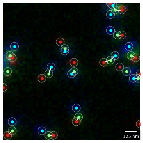
# the matches can be plotted
match.plot_match(channel_colors=["tab:red", "palegreen", "cyan"], circle_alpha=0.5)

# And the multicolor image can be plotted in the background
ax = plt.gca()

background_image, _, __ = multichannel_to_rgb(images=[image_A, image_B, image_C], cmaps=['pure_red','pure_green', 'pure_blue'])
ax.imshow(background_image)
ax.axis("off")
scalebar = ScaleBar(0.04,
        "nm",
        length_fraction=0.10,
        box_color="black",
        color="white",
        location="lower right")
scalebar.dx = 25
ax.add_artist(scalebar)

# we can chose to focus only on a section of the image by setting the limits 
plt.xlim([80, 140])
plt.ylim([80, 140])

plt.tight_layout()
plt.show()

w_ABC : 251 w_AB : 175 w_BC : 172 w_A : 211 w_B : 52 w_C : 260

You can interactively modify the maximum matching radius, as shown in the provided example. This also allows you to plot the detected abundance count against the varying maximum matching distance.

References

Naas J, Nies G, Li H, Stoldt S, Schmitzer B, Jakobs S, Munk A. "MultiMatch: geometry-informed colocalization in multi-color super-resolution microscopy." Commun Biol 7, 1139 (2024). https://doi.org/10.1038/s42003-024-06772-8